Welcome to kerrpy’s documentation!
Contents:
Indices and tables
Testing
-
class
kerrpy.camera.Camera(r, theta, phi, focalLength, sensorShape, sensorSize, roll=0, pitch=0, yaw=0)[source] Pinhole camera placed near a Kerr black hole.
This class contains the necessary data to define a camera that is located on the coordinate system of a Kerr black hole.
-
r¶ double – Distance to the coordinate origin; i.e., distance to the black hole centre.
-
r2¶ double – Square of r.
-
theta¶ double – Inclination of the camera with respect to the black hole.
-
phi¶ double – Azimuth of the camera with respect to the black hole.
-
focalLength¶ double – Distance between the focal point (where every ray that reaches the camera has to pass through) and the focal plane (where the actual sensor/film is placed).
-
sensorSize¶ tuple – 2-tuple that defines the physical dimensions of the sensor in the following way: (Height, Width).
-
sensorShape¶ tuple – 2-tuple that defines the number of pixels of the sensor in the following way: (Number of rows, Number of columns).
-
pixelWidth¶ double – Width of one single pixel in physical units. It is computed as Number of columns / Sensor width.
-
pixelHeight¶ double – Height of one single pixel in physical units. It is computed as Number of rows / Sensor height.
-
speed¶ double – Speed of the camera, that follows a circular orbit around the black hole in the equatorial plane. It is computed using the formula (A.7) of Thorne’s paper.
-
roll¶ double – The roll angle of the CCD; i.e., the rotation angle of the CCD on its plane. Defaults to zero, that means the CCD is facing the black hole centre.
-
pitch¶ double – The pitch angle of the CCD; i.e., the above/below direction of looking. Defaults to zero, that means the CCD is facing the black hole centre.
-
yaw¶ double – The yaw angle of the CCD; i.e., the left/right direction of lookin. Defaults to zero, that means the CCD is facing the black hole centre.
-
__init__(r, theta, phi, focalLength, sensorShape, sensorSize, roll=0, pitch=0, yaw=0)[source] Builds the camera defined by focalLength, sensorShape and sensorSize and locates it at the passed coordinates \((r_c, \theta_c, \phi_c)\)
Parameters: - r (double) – Distance to the coordinate origin; i.e., distance to the black hole centre.
- theta (double) – Inclination of the camera with respect to the black hole.
- phi (double) – Azimuth of the camera with respect to the black hole.
- focalLength (double) – Distance between the focal point (where every row that reaces the camera has to pass through) and the focal plane (where the actual sensor/film is placed).
- sensorShape (tuple) – 2-tuple that defines the number of pixels of the sensor in the following way: (Number of rows, Number of columns).
- sensorSize (tuple) – 2-tuple that defines the physical dimensions of the sensor in the following way: (Height, Width).
- roll (double) – The roll angle of the CCD; i.e., the rotation angle of the CCD on the plane of the CCD. Defaults to zero, that means the CCD is facing the black hole centre.
- pitch (double) – The pitch angle of the CCD; i.e., the above/below direction of looking. Defaults to zero, that means the CCD is facing the black hole centre.
- yaw (double) – The yaw angle of the CCD; i.e., the left/right direction of lookin. Defaults to zero, that means the CCD is facing the black hole centre.
-
__weakref__ list of weak references to the object (if defined)
-
-
class
kerrpy.raytracer.RayTracer(camera, debug=False)[source] Relativistic spacetime ray tracer.
This class generates images of what an observer would see near a rotating black hole.
This is an abstraction layer over the CUDA kernel that integrates the ODE system specified in equations (A.15) of Thorne’s paper. It integrates, backwards in time, a set of rays near a Kerr black hole, computing its trajectories from the focal point of a camera located near the black hole.
The RayTracer class hides all the black magic behind the CUDA code, giving a nice and simple interface to the user that just wants some really cool, and scientifically accurate, images.
Given a scene composed by a camera, a Kerr metric and a black hole, the RayTracer just expects a time \(x_{end}\) to solve the system.
Example
Define the characteristics of the black hole and build it:
spin = 0.9999999999
innerDiskRadius = 9
outerDiskRadius = 20
blackHole = BlackHole(spin, innerDiskRadius, outerDiskRadius)
Define the specifications of the camera and build it:
camR = 30
camTheta = 1.511
camPhi = 0
camFocalLength = 3
camSensorShape = (1000, 1000)  # (Rows, Columns)
camSensorSize = (2, 2)         # (Height, Width)
camera = Camera(camR, camTheta, camPhi,
                camFocalLength, camSensorShape, camSensorSize)
Create a Kerr metric with the previous two objects:
kerr = KerrMetric(camera, blackHole)
Set the speed of the camera once the Kerr metric and the black hole are created: it needs some info from both of these objects:
camera.setSpeed(kerr, blackHole)
Finally, build the raytracer with the camera, the metric and the black hole...:
rayTracer = RayTracer(camera, kerr, blackHole)
...and generate the image!:
rayTracer.rayTrace(-90)
rayTracer.synchronise()
rayTracer.plotImage()
-
__weakref__ list of weak references to the object (if defined)
-
rayTrace(xEnd, kernelCalls=1)[source] Parameters: - xEnd (float) – Time in which the system will be integrated. After this method finishes, the value of the rays at t=xEnd will be known
- stepsPerKernel (integer) – The number of steps each kernel call will compute; i.e., the host will call the kernel xEnd / (resolution*stepsPerKernel) times.
- resolution (float) – The size of the interval that will be used to compute one solver step between successive calls to the collision detection method.
-
texturedImage(disk, sphere)[source] Image should be a 2D array where each entry is a 3-tuple of Reals between 0.0 and 1.0
-
This is a test to know whether the figure automatic numbering really works. See Fig. 1 if everything’s fine.
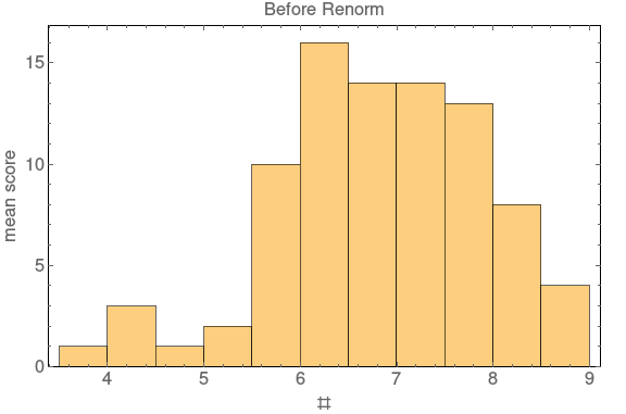
Fig. 1 This is the caption of the figure (a simple paragraph).
Doxygen testing
This file implements two numerical solvers for systems of N first order ordinary differential equations (y’ = F(x,y)).
The first solver, implemented in SolverRK45 and originally called DOPRI5, is described in [HNW93] and [HW96]. Specifically, see Table 5.2 [HNW93] for the Butcher’s table and Section II.4, subsection “Automatic Step Size Control” [HNW93], for the automatic control of the solver inner step size. See also Section IV.2 [HW96] for the stabilized algorithm. The second solver, SolverRK45, is adapted from [Cha16], and described at [CPO13].
Given an ODEs system, a matrix of initial conditions, each one of the form \( (x_0, y_0) \), and an interval \( [x_0, x_{end}] \), this code computes the value of the system at \( x_{end} \) for each one of the initial conditions. The computation is GPU parallelized using CUDA.
Functions
-
__device__ static Real
advanceStep(Real *y0, Real h, Real *y1, Real *data)¶ This method uses DOPRI5 to advance a time of
hthe system stored iny0. It reads the system state passed asy0, advance it using the stephand stores the result iny1. The last parameter, data, is used by the rhs of the system.- Return
- The normalized estimated error of the step.
- Parameters
y0: Initial state of the system.h: Step that shall be advanced.y1: Final state of the system,data: Additional data used by the rhs of the system.
-
__device__ int
bisect(Real *yOriginal, Real *data, Real step, Real x)¶ This function receives the current state of a ray that has just crossed the equatorial plane (theta = pi/2) and makes a binary search of the exact (with a tolerance of BISECT_TOL) point in which the ray crossed it. This code expects the following:
- In time = x, the ray is at one side of the equatorial plane.
- In time = x - step, the ray was at the opposite side of the equatorial plane.
- Return
- Number of iterations used in the binary search.
- Parameters
yOriginal: Pointer to the array where the ray state is stored, following the usual order used throughout this code: r, theta, phi, pR and pTheta.data: Device pointer to a serialized matrix of additional data to be passed to computeComonent; currently, this is used to pass the constants b and q of each ray to the computeComponent method.step: x - step was the last time in which the ray was found in the opposite side of the equatorial plane it is in the current time; i.e., at time = x.x: Current time.
-
__device__ int
SolverRK45(Real *globalX0, Real xend, Real *initCond, Real hOrig, Real hmax, Real *data, int *iterations)¶ Applies the DOPRI5 algorithm over the system defined in the computeComponent function, using the initial conditions specified in
devX0anddevInitCond, and returning the solution found atxend.- Parameters
globalX0: Start of the integration interval [x_0, x_{end}]. At the output, this variable is set to the final time the solver reached.xend: End of the integration interval [x_0, x_{end}].initCond: Device pointer to a serialized matrix of initial conditions; i.e., given a 2D matrix of R rows and C columns, where every entry is an n-tuple of initial conditions (y_0[0], y_0[1], ..., y_0[n-1]), the vector pointed by devInitCond contains R*C*n serialized entries, starting with the first row from left to right, then the second one in the same order and so on. The elements of vector pointed by initCond are replaced with the new computed values at the end of the algorithm; please, make sure you will not need them after calling this procedure.hOrig: Step size. This code controls automatically the step size, but this value is taken as a test for the first try; furthermore, the method returns the last computed value of h to let the user know the final state of the solver.hmax: Value of the maximum step size allowed, usually defined as x_{end} - x_0, as we do not to exceed x_{end} in one iteration.data: Device pointer to a serialized matrix of additional data to be passed to computeComonent; currently, this is used to pass the constants b and q of each ray to the computeComponent method.iterations: Output variable to know how many iterations were spent in the computation
Functions
-
__device__ void
getCanonicalMomenta(Real rayTheta, Real rayPhi, Real *pR, Real *pTheta, Real *pPhi)¶ Given the ray’s incoming direction on the camera’s local sky, rayTheta and rayPhi, this function computes its canonical momenta. See Thorne’s paper, equation (A.11), for more information. Note that the computation of this quantities depends on the constants __camBeta (speed of the camera) and __ro, __alpha, __omega, __pomega and __ro (Kerr metric constants), that are defined in the common.cu template.
- Parameters
rayTheta: Polar angle, or inclination, of the ray’s incoming direction on the camera’s local sky.rayPhi: Azimuthal angle, or azimuth, of the ray’s incoming direction on the camera’s local sky.pR: Computed covariant coordinate r of the ray’s 4-momentum.pTheta: Computed covariant coordinate theta of the ray’s 4-momentum.pPhi: Computed covariant coordinate phi of the ray’s 4-momentum.
-
__device__ void
getConservedQuantities(Real pTheta, Real pPhi, Real *b, Real *q)¶ Given the ray’s canonical momenta, this function computes its constants b (the axial angular momentum) and q (Carter constant). See Thorne’s paper, equation (A.12), for more information. Note that the computation of this quantities depends on the constant __camTheta, which is the inclination of the camera with respect to the black hole, and that is defined in the common.cu template
- Parameters
pTheta: Covariant coordinate theta of the ray’s 4-momentum.pPhi: Covariant coordinate phi of the ray’s 4-momentum.b: Computed axial angular momentum.q: Computed Carter constant.
-
__global__ void
setInitialConditions(void *devInitCond, void *devConstants, Real pixelWidth, Real pixelHeight)¶ CUDA kernel that computes the initial conditions (r, theta, phi, pR, pPhi) and the constants (b, q) of every ray in the simulation.
This method depends on the shape of the CUDA grid: it is expected to be a 2D matrix with at least IMG_ROWS threads in the Y direction and IMG_COLS threads in the X direction. Every pixel of the camera is assigned to a single thread that computes the initial conditions and constants of its corresponding ray, following a pinhole camera model.
Each thread that executes this method implements the following algorithm:
- Compute the pixel physical coordinates, considering the center of the sensor as the origin and computing the physical position using the width and height of each pixel.
- Compute the ray’s incoming direction, theta and phi, on the camera’s local sky, following the pinhole camera model defined by the sensor shape and the focal distance __d.
- Compute the canonical momenta pR, pTheta and pPhi with the method
getCanonicalMomenta. - Compute the ray’s constants b and q with the method.
getConservedQuantities. - Fill the pixel’s corresponding entry in the global array pointed by devInitCond with the initial conditions: __camR, __camTheta, __camPhi, pR and pTheta, where the three first components are constants that define the position of the focal point on the black hole coordinate system.
- Fill the pixel’s corresponding entry in the global array pointed by devConstants with the computed constants: b and q.
- Parameters
devInitCond: Device pointer to a serialized 2D matrix where each entry corresponds to a single pixel in the camera sensor. If the sensor has R rows and C columns, the vector pointed by devInitCond contains R*C entries, where each entry is a 5-tuple prepared to receive the initial conditions of a ray: (r, theta, phi, pR, pPhi). At the end of this kernel, the array pointed by devInitCond is filled with the initial conditions of every ray.devConstants: Device pointer to a serialized 2D matrix where each entry corresponds to a single pixel in the camera sensor. If the sensor has R rows and C columns, the vector pointed by devConstants contains R*C entries, where each entry is a 2-tuple prepared to receive the constants of a ray: (b, q). At the end of this kernel, the array pointed by devConstants is filled with the computed constants of every ray.pixelWidth: Width, in physical units, of the camera’s pixels.pixelHeight: Height, in physical units, of the camera’s pixels.
-
__global__ void
kernel(Real x0, Real xend, void *devInitCond, Real h, Real hmax, void *devData, void *devStatus, Real resolutionOrig)¶ CUDA kernel that integrates a set of photons backwards in time from x0 to xend, storing the final results of their position and canonical momenta on the array pointed by devInitCond.
This method depends on the shape of the CUDA grid: it is expected to be a 2D matrix with at least IMG_ROWS threads in the Y direction and IMG_COLS threads in the X direction. Every ray is assigned to a single thread, which computes its final state solving the ODE system defined by the relativistic spacetime.
Each thread that executes this method implements the following algorithm:
- Copy the initial conditions and constants of the ray from its corresponding position at the global array devInitCond and devData into local memory.
- Integrate the ray’s equations defined in Thorne’s paper, (A.15). This is done while continuosly checking whether the ray has collided with disk or horizon.
- Overwrite the conditions at devInitCond to the new computed ones. Fill the ray’s final status (no collision, collision with the disk or collision with the horizon) in the devStatus array.
- Parameters
x0: Start of the integration interval [x_0, x_{end}]. It is usually zero.xend: End of the integration interval [x_0, x_{end}].devInitCond: Device pointer to a serialized 2D Real matrix where each entry corresponds to a single pixel in the camera sensor; i.e., to a single ray. If the sensor has R rows and C columns, the vector pointed by devInitCond contains R*C entries, where each entry is a 5-tuple filled with the initial conditions of the corresponding ray: (r, theta, phi, pR, pPhi). At the end of this kernel, the array pointed by devInitCond is overwritten with the final state of each ray.h: Step size for the Runge-Kutta solver.hmax: Value of the maximum step size allowed in the Runge-Kutta solver.devData: Device pointer to a serialized 2D Real matrix where each entry corresponds to a single pixel in the camera sensor; i.e., to a single ray. If the sensor has R rows and C columns, the vector pointed by devData contains R*C entries, where each entry is a 2-tuple filled with the constants of the corresponding ray: (b, q).devStatus: Device pointer to a serialized 2D Int matrix where each entry corresponds to a single pixel in the camera sensor; i.e., to a single ray. If the sensor has R rows and C columns, the vector pointed by devData contains R*C entries, where each entry is an integer that will store the ray’s status at the end of the kernelresolutionOrig: Amount of time in which the ray will be integrated without checking collisions. The lower this number is (in absolute value, as it should always be negative), the more resolution you’ll get in the disk edges.
Functions
-
__global__ void
generate_textured_image(void *devRayCoordinates, void *devStatus, void *devImage)
-
__global__ void
generate_image(void *devRayCoordinates, void *devStatus, void *devDiskTexture, int diskRows, int diskCols, void *devSphereTexture, int sphereRows, int sphereCols, void *devImage)
Defines
-
__FUNCTIONS__
Functions
-
__device__ void
computeComponent(Real *y, Real *f, Real *data)¶ Computes the value of the function F(t) = (dr/dt, dtheta/dt, dphi/dt, dpr/dt, dptheta/dt) and stores it in the memory pointed by f.
- Parameters
y: Initial conditions for the system: a pointer to a vector whose lenght shall be the same as the number of equations in the system: 5f: Computed value of the function: a pointer to a vector whose lenght shall be the same as the number of equations in the system: 5data: Additional data needed by the function, managed by the caller. Currently used to get the ray’s constants b and q.
doxygenfunction:: advanceStep
Bibliography
| [Cha16] | Chi Kwan Chan. A massive parallel ode integrator for performing general relativistic radiative transfer using ray tracing. https://github.com/chanchikwan/gray, 2016. |
| [CPO13] | Chi Kwan Chan, Dimitrios Psaltis, and Feryal Ozel. Gray: a massively parallel gpu-based code for ray tracing in relativistic spacetimes. The Astrophysical Journal, 2013. arXiv:arXiv:1303.5057, doi:10.1088/0004-637X/777/1/13. |
| [HNW93] | (1, 2, 3) Ernst Hairer, Syvert P. Nørsett, and Gerhard Wanner. Solving Ordinary Differential Equations I. volume 8 of Springer Series in Computational Mathematics. Springer-Verlag Berlin Heidelberg, Berlin New York, 1993. ISBN 978-3-540-56670-0. |
| [HW96] | (1, 2) Ernst Hairer and Gerhard Wanner. Solving Ordinary Differential Equations II. volume 14 of Springer Series in Computational Mathematics. Springer-Verlag Berlin Heidelberg, Berlin New York, 1996. ISBN 978-3-642-05220-0. |